Appendix
A Architecture
The model is a decoder-only transformer of the modded-nanoGPT kind: eight pre-norm blocks of width 512 with eight heads, RMS normalization, rotary position embeddings with normalized queries and keys, a squared-ReLU MLP of width 2048, and no biases. Attention is causal with a sliding window of 1024 tokens in three of every four blocks and the full 2048 in the others. Every other block adds a value embedding to its values, a second token embedding scaled per head by a learned gate on the block input. The residual stream entering each block is a learned mix of the previous block’s output and the token embedding, and these $2L$ mixing scalars are the parameters trained by weight-space ES. The head is untied, with capped logits. Token and value embeddings are stored in bfloat16 and the forward runs in bfloat16. The base model has 37.7M parameters; the model-size study uses two, four and sixteen blocks of width 128, 256 and 1024, with the same head dimension.
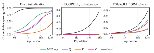
B Cosine Ladder at the Remaining Checkpoints
C Test Losses by Token Budget and Population
Table 1 has the test losses behind Figure 2.
| Population | 100k | 1M | 10M | 20M | |
|---|---|---|---|---|---|
| Dust | 64 | 7.240 | 6.290 | 5.397 | 5.265 |
| 256 | 7.165 | 6.067 | 5.231 | 5.139 | |
| 1k | 7.151 | 5.934 | 5.111 | 4.960 | |
| 4k | 7.164 | 5.911 | 5.072 | 4.912 | |
| 16k | 7.170 | 5.916 | 5.049 | 4.802 | |
| $\infty$ (fit) | 7.161 | 5.892 | 5.013 | 4.431 | |
| EGGROLL | 64 | 7.961 | 7.428 | 7.056 | 6.987 |
| 256 | 7.605 | 7.200 | 6.906 | 6.811 | |
| 1k | 7.386 | 7.046 | 6.692 | 6.517 | |
| 4k | 7.302 | 6.892 | 6.352 | 6.200 | |
| 16k | 7.263 | 6.708 | 6.033 | 5.865 | |
| Backprop | 7.216 | 5.959 | 4.989 | 4.633 |
D EGGROLL’s Extrapolated Population
We extrapolate EGGROLL’s ladder at 1M tokens and more to the population at which it would match Dust at 64 draws (Section 3.2). Table 2 gives that population as a multiple of 64 under three fits of EGGROLL’s cells in Table 1. The power law is the fit of Figure 2, $L(P) = A P^{-\alpha} + E$, which we also refit with each population left out in turn. The straight lines in log population are least-squares fits to the top three populations (1k, 4k and 16k) and the top two (4k and 16k). The three fits put the multiple between about 3,000 and 23,000.
| Fit | 1M | 10M | 20M |
|---|---|---|---|
| Power law, all five populations | 23,000$\times$ | 16,000$\times$ | 8,100$\times$ |
| Power law, one population left out | 11,000$\times$ to $\infty$ | 7,200$\times$ to 54,000$\times$ | 4,700$\times$ to 17,000$\times$ |
| Straight line in log population, top three | 8,200$\times$ | 3,700$\times$ | 3,300$\times$ |
| Straight line in log population, top two | 6,000$\times$ | 4,100$\times$ | 3,100$\times$ |
E Population Allocation
$K$ counts the draws rewarded with token losses. Table 3 lists everything an update jitters, with its draws at $K = 16{,}384$ and its noise scale, and Table 4 splits the three per-block streams over the blocks. Populations from 256 up scale every count by $K/16{,}384$. At 64 draws the recipe at 1M and 10M is $(8,7,4,3,1,1,1,1)$ writer draws, $(8,7,4,3,2,1,1,1)$ MLP draws, one attention-output draw per block, three embedding draws and 1, 5, 2, 3 and 2 draws for $q$, $v$, the gate, $k$ and the value embedding. The nominal stream ratio before rounding is $(\text{writers}+\text{MLP}):\text{attention outputs}:\text{embedding} = 7:0.75:0.25$ (at 100k tokens $6:1.5:0.5$), with a tilt toward the first blocks that comes from a coordinate descent over the allocation at 2k draws.
| Draws | ||||
|---|---|---|---|---|
| Site | One draw reruns | SGD | Adam | Noise scale |
| Writer pair | its block onward | 7,040 | 4,096 | 0.2 |
| MLP hidden layer | its block onward | 7,040 | 4,096 | 0.2 |
| Attention output | its block onward | 1,664 | 6,144 | 0.2, deeper half 0.4 |
| Token embedding | the whole network | 640 | 8,192 | 0.2, Adam 0.4 |
| Query, per block | its block’s attention | 128 | 128 | 0.05 |
| Value, per block | its block’s attention | 1,280 | 1,280 | 0.05 |
| Gate, per block | its block’s attention | 384 | 384 | 0.05 |
| Key, per block | its block’s attention | 768 | 768 | 0.05 |
| Value embedding, per block | its block’s attention | 512 | 512 | 0.05 |
| Head | one slab’s cross-entropy | 65,536 | 49,152 | 0.05 |
| Residual scalars | the whole network, twice | 8 | 8 | 0.03 |
| Writer pair, MLP hidden layer | Attention output | |||||||
|---|---|---|---|---|---|---|---|---|
| Block | 100k | 1M, 10M | 20M | 10M at 16k | 20M at 16k | 100k | all others | 10M at 16k |
| 1 | 2048 | 2432 | 2816 | 2176 | 2304 | 896 | 384 | 768 |
| 2 | 1792 | 2048 | 2432 | 1792 | 2048 | 768 | 384 | 640 |
| 3 | 896 | 1024 | 896 | 896 | 768 | 512 | 256 | 512 |
| 4 | 640 | 640 | 256 | 512 | 256 | 384 | 128 | 256 |
| 5 | 256 | 384 | 256 | 384 | 256 | 128 | 128 | 256 |
| 6 | 256 | 256 | 128 | 256 | 128 | 128 | 128 | 256 |
| 7 | 128 | 128 | 128 | 128 | 128 | 128 | 128 | 256 |
| 8 | 128 | 128 | 128 | 128 | 128 | 128 | 128 | 256 |
| Total | 6144 | 7040 | 7040 | 6272 | 6016 | 3072 | 1664 | 3200 |
Draws are evaluated $n$ at a time on one GPU, with $n = 1, 2, 8, 8, 16$ at $K = 64, 256, 1{,}024, 4{,}096, 16{,}384$, and split evenly across GPUs. Direct loss estimates and queries use $\gamma=0$. Keys, values, gates and value embeddings use $\gamma=0.99$ in the main comparison’s 10M/16k and 20M/16k runs, and $\gamma=0.98$ in all other runs. At 20M and 16k draws, $k$ and $v$ get 1,536 and 2,560 draws per block, so that cell has 14,336 draws rewarded with losses at the compute of the other 16k cells. For the other model sizes the tilt is sampled at the same relative depth and the attention-internal counts are scaled so that their totals match the 8-layer model.
F Tuning
Every cell of the main comparison, a token budget and a population for Dust and a token budget for backprop, is tuned the same way. Both methods tune momentum and learning rate only, starting from the grid of Table 5. Every other constant is fixed (Section 3.1, Appendix E), the learning rates of Table 6 included. Seed 42 runs the grid; the best point and every point within 0.02 of it get seeds 43 and 44, as does any point whose single seed beats the current three-seed best. A best point on the edge of the grid has the grid extended one step along its line until the best point is interior, and the two rate half-steps around it are then run under the same rules. A run whose final validation loss exceeds its best by more than 0.25, or that ever exceeds the uniform-prediction loss $\ln V$, or produces a NaN, is rejected together with its configuration. The selected configuration is the lowest mean validation loss over the three seeds, and we report its test loss at each seed’s best-validation checkpoint.
| Cells | Momentum | Learning rate |
|---|---|---|
| 100k tokens | 0.2, 0.3, 0.5 | 0.3, 0.4, 0.5, 0.6 |
| 1M, 10M and 20M tokens | 0.9, 0.95, 0.98 | 0.1, 0.15, 0.2, 0.25 |
| 10M tokens at 64 draws | 0.95, 0.98, 0.99 | 0.0125, 0.025, 0.05, 0.1 |
| 20M tokens at 64 draws | 0.95, 0.98, 0.99 | 0.00625, 0.0125, 0.025, 0.05 |
| Main comparison | Model-size study | |||
|---|---|---|---|---|
| Parameters | Dust | Backprop | Dust | Backprop |
| Key projections | base | base | $4\times$ base | $4\times$ base |
| Value projections | base | base | $8\times$ base | $8\times$ base |
| Token embedding | 1000 | 1000 | 0.3 | base |
| Value embeddings | 0.3 | base | 0.3 | base |
| Residual scalars | 0.03 | base | 0.03 | base |
| Everything else | base | base | base | base |
The overparameterization experiments were run before we improved the token-embedding learning rate. They use the earlier training settings in Table 6, which explains the difference from the main results.
Dust’s own constants, the noise scales, the credit decay and the draw allocation, are chosen with the cosine diagnostic of Section 2.3, confirmed in training, and held fixed across cells. At the 16k cells of 10M and 20M tokens they are tuned in training together with momentum and rate at fixed compute: each lever, the allocation across layer families, the per-block tilt, the noise scales, the credit decay and the head draws, is run one at a time from the (momentum, rate) winner, seeded in stages on wins paired by seed, and the winning levers are stacked; backprop receives the same wider (momentum, rate) grid at three seeds. The selected constants are those of Appendix E. Not every lever ran at 20M within the campaign, and the other cells keep the constants from the cosine tuning, so at those two budgets the top cell of the ladder has constants of its own, which the 10M fit is read with.
Under Adam, three learning-rate groups, matrices and the head, token and value embeddings, and residual mixing scalars, are tuned for Dust and backprop. Table 7 has the selected settings at 1M tokens.
| Dust | Backprop | EGGROLL | |
|---|---|---|---|
| Matrices and head, at 64 draws | 0.00175 | 0.002 | 0.003 |
| Matrices and head, from 256 to 4k | 0.0015 | 0.002 | 0.003 |
| Matrices and head, from 16k up | 0.002 | 0.002 | 0.003 |
| Token and value embeddings | $300\times$ matrices | 0.3 | 0.003 |
| Residual scalars | $100\times$ matrices | 0.2 | 0.003 |
| $\beta_1$ | 0.7 | 0.8 | 0.5 |
The model-size study of Section 4.1 changes two hyperparameters from Section 3 (Table 6). The token embedding stays at its default learning rate, 0.3 for Dust and the base rate for backprop, because at 1000 backprop shows no clear separation between model sizes, which makes overparameterization hard to study. We also keep the key and value learning rates of the earlier protocol and tune them for both Dust and backprop, so the comparison is fair to both.
G Cosine-fit parameters
Table 8 reports fits of $C(K) = c_{\max}/\sqrt{1+c/K}$ to measured cosine similarities at the final 100M token checkpoint. Each fit uses seven population budgets from 64 to 131072. At each budget, cosine similarity is computed separately for each weight matrix and then averaged across matrices of the same layer type. The fitted parameter $c$ uses the same population-budget units as $K$, rather than the individual draw count of a particular layer. RMSE is computed across the seven measured points used for fitting.
| Layer type | $c_{\max}$ | $c$ | RMSE |
|---|---|---|---|
| 100M-token checkpoint | |||
| MLP out | 0.8779 | 31623 | 0.0081 |
| MLP in | 0.8577 | 48417 | 0.0065 |
| Attn out | 0.8729 | 21627 | 0.0093 |
| Attn Q | 1.0000 | 76736 | 0.0356 |
| Attn K | 1.0000 | 616595 | 0.0191 |
| Attn V | 0.8776 | 173780 | 0.0269 |
| Value gate | 0.6657 | 47863 | 0.0367 |
| Value emb | 1.0000 | 495450 | 0.0247 |
| Token emb | 0.7318 | 19498 | 0.0083 |
| LM head | 1.0000 | 759 | 0.0032 |